Upgrade to the Modern Data Stack

 

Solution: The Modern Data Stack

There's already a tool perfectly suited to storing massive amounts of data, that can be queried easily, and is connected to everything. A database or data warehouse. You probably already have one running in your company that you can reuse so you don't need to buy another CRM, CDP, DMP, MAP, or any other acronym.

Building around a data warehouse has additional benefits such as:

• You own your data. It helps you comply with different regulations.
• Get value quicker. It is 10x easier to dump historical data in a DB than importing the data in yet-another-tool.
• Easier to sync with other tools. Databases integrate with everything, contrary to SaaS Tools that have limited APIs (and please don't get me started on APIs like Marketo).
• Reusability. Other teams in the company can use this trusted source of truth.

In addition to a data warehouse, you will need 4 other key components:

1. An event tracking tool. You can continue using Segment here. It does the job well and allows you to collect events across all of your websites & apps.
2. A data loader. I recommend Fivetran. It’s easy to set up in a couple of clicks and amazingly reliable.
3. A data modeling tool. DBT is the new power tool here. It allows you to transform and model your data.
4. An Integration Platform. I’m a 100% biased here, but I recommend using Census. We integrate well with DBT and enable you to sync your clean and unified data models back to all of your other tools.

As a bonus, you can replace Amplitude with a BI tool like Mode or Chart.io, which is cheap and as good as Looker.

Reference: https://www.getcensus.com/blog/graduating-to-the-modern-data-stack-for-startups

Modern data stack - 2021 and beyond

Modern Data Stack -  2021 and beyond

Product analytics and the modern tech stack

References:

https://mixpanel.com/blog/product-analytics-and-the-modern-tech-stack/

https://snowplowanalytics.com/blog/2021/05/12/modern-data-stack/

Open Source Miracles : ClickHouse

ClickHouse is a free analytics DBMS for big data. It is an open-source column-oriented database management system that allows generating analytical data reports in real-time.

Reference:

Github: https://github.com/ClickHouse/ClickHouse

Usecases: https://clickhouse.com/use-cases/

When to use Airbyte along with Airflow

 When to use Airbyte along with Airflow?

Airflow shines as a workflow orchestrator. Because Airflow is widely adopted, many data teams also use Airflow transfer and transformation operators to schedule and author their ETL pipelines. Several of those data teams have migrated their ETL pipelines to follow the ELT paradigm. We have seen some of the challenges of building full data replication and incremental loads DAGs with Airflow. More troublesome is that sources and destinations are tightly coupled in Airflow transfer operators. Because of this, it will be hard for Airflow to cover the long-tail of integrations for your business applications. 

One alternative is to keep using Airflow as a scheduler and integrate it with two other open-source projects that are better suited for ELT pipelines, Airbyte for the EL parts and dbt for the T part. Airbyte sources are decoupled from destinations so you can already sync data from 100+ sources (databases,  APIs, ...) to 10+ destinations (databases, data warehouses, data lakes, ...) and remove boilerplate code needed with Airflow. With dbt you can transform data with SQL in your data warehouse and avoid having to handle dependencies between tables in your Airflow DAGs.

References:

Airbyte https://github.com/airbytehq/airbyte

Airflow https://airbyte.io/blog/airflow-etl-pipelines

dbt https://github.com/dbt-labs/dbt-core

dbt implementation at Telegraph https://medium.com/the-telegraph-engineering/dbt-a-new-way-to-handle-data-transformation-at-the-telegraph-868ce3964eb4

Internal architecture and design of Snowflake!

Have you ever wondered how Snowflake has designed their elastic data warehouse, then here is an extremely nice read to know more details about it?

Reference: http://info.snowflake.net/rs/252-RFO-227/images/Snowflake_SIGMOD.pdf

Open Source Miracles : NocoDB

NocoDB is an Open Source Airtable Alternative, and it turns any MySQL, PostgreSQL, SQL Server, SQLite & MariaDB into a smart spreadsheet.

It has the following rich features

• Smartsheet features such as search, views, filters, roles and permissions and etc
• Upload images to major storage cloud providers
• Workflow automation which includes alerts, notifications and etc
• Programmatic API features such as Swagger, GraphQA and etc

Reference: https://github.com/nocodb/nocodb 

Why Digital is The Future! How to have a successful journey...

Why Digital is The Future! How to have a successful journey...

"Digital" and "digitization" or "online" has become a very common word in the recent past due to the C-19 pandemic situation, and yet, the digital transformation has been there in every industry more than two decades or so to create value-driven business opportunities for the organizations in their served customer segments with the right value proposition to fulfill their internal and external customers with amazing customer experiences (CX).

Some basics to know- The average IT spend across all industries was around 8 percent of their revenues as a magic number and yet it depends on many factors like industry, region, and age of the company, etc. Now, think about organizations spending between 4 to 24 percent based on the industry for their IT or digital goals, wherein the staff of IT and CIO or CDO would be bringing seamless and easy to use tools and solutions for the various businesses including sales and markets and other business functions in the company (plus external customers too). 

On a side note, usually, companies spend roughly around 10 percent as a magic number on sales and marketing, with a disclaimer that it depends on the size of the company and which sector it belongs to, etc.

With that, it's very imperative that you as a CTO or CDO or CIO or Digital IT Head need to have a very clear plan to create a successful journey towards it with the available budgets in place... 

Some of the key caveats for the success of any organization to become truly digital are:

• Make sure to address the five domains of the digital strategy - customers, competition, data, innovation, and value
• Create a comprehensive digital platform with digital products, and not siloed or isolated apps or customizations
• Start with small to focus more on the CX, and then slowly evolve and improvise your design
• How fast you pivot to digital is the clear caveat to bring more efficiencies and value to your businesses and their respective functions
• Have a clear business architecture and enterprise architecture in place whenever your organization do any M&As and adapt as quickly as possible so that all the respective fulfillment happens seamlessly for the existing (for example, legacy apps) and newly acquired customers
• Application and/or software modernization with the latest emerging technologies like microservices, cloud, machine learning, artificial intelligence, monitoring, cybersecurity, etc
• IT architecture is very important to any organization, and yet, that needs to be refined every now and then to meet your business outcomes and demands
• Having an application rationalization chart to know the right sunset and sunrise digital products based on your organization priorities so that it is easier to maintain and innovate faster while the systems and applications are co-existing with newer digital products; a clear winner to achieve improvements in business operations
• Always, treat your data as the biggest asset to your organization to do any sort of transformation and decision making
• Make sure to have highly available, reliable, and accurate data APIs/Services for the key source of truth from the various data stores, these can be called as DaaS (Data as a Service) to ease accessibility and minimize the data issues
• A robust operational backbone is necessary but that certainly is not sufficient for an organization's digital future, an organization needs to adapt to the newer technologies and have to innovate faster to create newer digital products or try to leverage existing newer COTS (Commercial off-the-shelf) tools to create newer digital solutions to continue delight and address all of your customer behaviors
• Always, have shared data analytics or insights from the data that you have collected from customers
• Re-use, Re-design, and Re-create wherever and whenever required to save time and money
• Have intelligent automation in place for automating some/many of the most used business processes
• Promote continuous delivery and/or integration with DevOps and SRE (Site reliability engineering) principles, so that feedback loops/cycles are faster and teams can implement and address them in a nimble fashion
• Promote co-creations and co-ownerships with the right internal and external accountability frameworks with faster pace decision making and approvals etc
• "digital" is everyone's job to become truly a digital organization. For example, to have the right business owners or product owners and then create more collaborative and agile ways of working together to reduce risks and dependencies
• Try to create a mindset where the customer is more important than anything, and providing seamless customer experience matters a lot
• Treat your tech debt as an innovation aspect of the digital journey, and have the organizational culture as design thinking instead of leaner thinking to come up with innovative digital solutions
• Having a digital product mindset instead of a project mindset
• Also, an organization can focus mostly on their core foundations and innovation only by having a great powerful external partner and/or developer community who gives you early feedbacks and promote your organization with ever scaling digital platforms
• Have resiliency aspects in your planned mission-critical releases, plan very well for the unplanned occurrences, and have architecture design for the next billion users

References/books:

Enterprise Architecture As Strategy: Creating a Foundation for Business Execution

Designed for Digital: How to Architect Your Business for Sustained Success (Management on the Cutting Edge)

Why Digital Transformations Fail: The Surprising Disciplines of How to Take Off and Stay Ahead

The Lean Product Playbook: How to Innovate with Minimum Viable Products and Rapid Customer Feedback

https://www.amazon.com/Enterprise-Architecture-Strategy-Foundation-Execution/dp/1591398398

https://www.bmc.com/blogs/digital-transformation-books/

https://www.cnbc.com/2019/04/08/4-trillion-in-tech-spending-in-2019-heres-where-the-money-is-going.html

https://vtldesign.com/digital-marketing/content-marketing-strategy/percent-of-revenue-spent-on-marketing-sales/

https://www.flexera.com/blog/elo/2020-state-of-tech-spend-it-spending-benchmarks-and-trends/

https://www.flexera.com/blog/industry-trends/it-spending-by-industry/

https://blog.techvera.com/company-it-spend

Database migrations aren't tough; use the right tools

Database migrations are not tough and it's all about how you use the right tools to overcome your most common issues for your on-going database development changes.

Most famous open source tools are:

1. https://www.liquibase.org/
2. https://flywaydb.org/
3. Many more...

So, what to choose and when to use liquibase vs. flyway

• liquibase and flyway has more or less same features, except the flyway uses the SQL as a script whereas liquibase supports SQL, YAML, XML, JSON
• Easier setup and configurations then, flyway; liquibase also easy setup though
• Both flyway and liquibase have tooling and integrations support with your CI/CD tech stack
• Little more configurations with more features you need then, go for liquibase 
• liquibase has a lot of databases supported
• liquibase has database versions controlling
• liquibase has undoing the migrations, and doing the diff etc whereas, it's premium in flyway
• smaller teams and many projects then, go flyway
• bigger teams with many projects then go for liquibase as you can have rollback and diff features as all varieties of scripts can be supported

References:

https://medium.com/@ruxijitianu/database-version-control-liquibase-versus-flyway-9872d43ee5a4

https://github.com/flyway/flyway

https://github.com/liquibase/liquibase

Most common ML Algorithms explained in a nutshell

Most common ML Algorithms explained in a nutshell

The prevalence of machine learning has been increasing tremendously in recent years due to the high demand and advancements in technology. The potential of machine learning to create value out of data has made it appealing for businesses in many different industries. Most machine learning products are designed and implemented with off-the-shelf machine learning algorithms with some tuning and minor changes.

There is a wide variety of machine learning algorithms that can be grouped in three main categories:

• Supervised learning algorithms model the relationship between features (independent variables) and a label (target) given a set of observations. Then the model is used to predict the label of new observations using the features. Depending on the characteristics of target variable, it can be a classification (discrete target variable) or a regression (continuous target variable) task.
• Unsupervised learning algorithms try to find the structure in unlabeled data.
• Reinforcement learning works based on an action-reward principle. An agent learns to reach a goal by iteratively calculating the reward of its actions.

In this post, I will cover the most common algorithms in the first two categories.

Note: Although deep learning is a sub-field of machine learning, I will not include any deep learning algorithms in this post. I think deep learning algorithms should be discussed separately due to complexity and having distinct dynamics. Besides, I hesitate to make this post too long and bore the readers.

Let’s start.

1. Linear Regression

Linear regression is a supervised learning algorithm and tries to model the relationship between a continuous target variable and one or more independent variables by fitting a linear equation to the data.

For a linear regression to be a good choice, there needs to be a linear relation between independent variable(s) and target variable. There are many tools to explore the relationship among variables such as scatter plots and correlation matrix. For example, the scatter plot below shows a positive correlation between an independent variable (x-axis) and dependent variable (y-axis). As one increases, the other one also increases.

A linear regression model tries to fit a regression line to the data points that best represents the relations or correlations. The most common technique to use is ordinary-least squares (OLE). With this method, best regression line is found by minimizing the sum of squares of the distance between data points and the regression line. For the data points above, the regression line obtained using OLE seems like:

---

2. Support Vector Machine

Support Vector Machine (SVM) is a supervised learning algorithm and mostly used for classification tasks but it is also suitable for regression tasks.

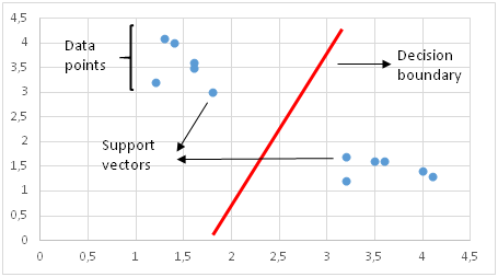
SVM distinguishes classes by drawing a decision boundary. How to draw or determine the decision boundary is the most critical part in SVM algorithms. Before creating the decision boundary, each observation (or data point) is plotted in n-dimensional space. “n” is the number of features used. For instance, if we use “length” and “width” to classify different “cells”, observations are plotted in a 2-dimensional space and decision boundary is a line. If we use 3 features, decision boundary is a plane in 3-dimensional space. If we use more than 3 features, decision boundary becomes a hyperplane which is really hard to visualize.

Decision boundary in 2D space is a line

Decision boundary is drawn in a way that the distance to support vectors are maximized. If the decision boundary is too close to a support vector, it will be highly sensitive to noises and not generalize well. Even very small changes in independent variables may cause a misclassification.

The data points are not always linearly separable like in the figure above. In these cases, SVM uses kernel trick which measures the similarity (or closeness) of data points in a higher dimensional space in order to make them linearly separable.

Kernel function is kind of a similarity measure. The inputs are original features and the output is a similarity measure in the new feature space. Similarity here means a degree of closeness. It is a costly operation to actually transform data points to a high-dimensional feature space. The algorithm does not actually transform the data points to a new, high dimensional feature space. Kernelized SVM compute decision boundaries in terms of similarity measures in a high-dimensional feature space without actually doing a transformation. I think this is why it is also called kernel trick.

SVM is especially effective in cases where number of dimensions are more than the number of samples. When finding the decision boundary, SVM uses a subset of training points rather than all points which makes it memory efficient. On the other hand, training time increases for large datasets which negatively effects the performance.

---

3. Naive Bayes

Naive Bayes is a supervised learning algorithm used for classification tasks. Hence, it is also called Naive Bayes Classifier.

Naive bayes assumes that features are independent of each other and there is no correlation between features. However, this is not the case in real life. This naive assumption of features being uncorrelated is the reason why this algorithm is called “naive”.

The intuition behind naive bayes algorithm is the bayes’ theorem:

p(A|B): Probability of event A given event B has already occurred

p(B|A): Probability of event B given event A has already occuured

p(A): Probability of event A

p(B): Probability of event B

Naive bayes classifier calculates the probability of a class given a set of feature values (i.e. p(yi | x1, x2 , … , xn)). Input this into Bayes’ theorem:

p(x1, x2 , … , xn | yi) means the probability of a specific combination of features (an observation / row in a dataset) given a class label. We need extremely large datasets to have an estimate on the probability distribution for all different combinations of feature values. To overcome this issue, naive bayes algorithm assumes that all features are independent of each other. Furthermore, denominator (p(x1,x2, … , xn)) can be removed to simplify the equation because it only normalizes the value of conditional probability of a class given an observation ( p(yi | x1,x2, … , xn)).

The probability of a class ( p(yi) ) is very simple to calculate:

Under the assumption of features being independent, p(x1, x2 , … , xn | yi) can be written as:

The conditional probability for a single feature given the class label (i.e. p(x1 | yi) ) can be more easily estimated from the data. The algorithm needs to store probability distributions of features for each class independently. For example, if there are 5 classes and 10 features, 50 different probability distributions need to be stored.

Adding all these up, it became an easy task for naive bayes algorithm to calculate the probability to observe a class given values of features (p(yi | x1, x2 , … , xn) )

The assumption that all features are independent makes naive bayes algorithm very fast compared to complicated algorithms. In some cases, speed is preferred over higher accuracy. On the other hand, the same assumption makes naive bayes algorithm less accurate than complicated algorithms. Speed comes at a cost!

---

4. Logistic Regression

Logistic regression is a supervised learning algorithm which is mostly used for binary classification problems. Although “regression” contradicts with “classification”, the focus here is on the word “logistic” referring to logistic function which does the classification task in this algorithm. Logistic regression is a simple yet very effective classification algorithm so it is commonly used for many binary classification tasks. Customer churn, spam email, website or ad click predictions are some examples of the areas where logistic regression offers a powerful solution.

The basis of logistic regression is the logistic function, also called the sigmoid function, which takes in any real valued number and maps it to a value between 0 and 1.

Consider we have the following linear equation to solve:

Logistic regression model takes a linear equation as input and uses logistic function and log odds to perform a binary classification task. Then, we will get the famous s shaped graph of logistic regression:

We can use the calculated probability ‘as is’. For example, the output can be “the probability that this email is spam is 95%” or “the probability that customer will click on this ad is 70%”. However, in most cases, probabilities are used to classify data points. For instance, if the probability is greater than 50%, the prediction is positive class (1). Otherwise, the prediction is negative class (0).

It is not always desired to choose positive class for all probability values higher than 50%. Regarding the spam email case, we have to be almost sure in order to classify an email as spam. Since emails detected as spam directly go to spam folder, we do not want the user to miss important emails. Emails are not classified as spam unless we are almost sure. On the other hand, when classification in a health-related issue requires us to be much more sensitive. Even if we are a little suspicious that a cell is malignant, we do not want to miss it. So the value that serves as a threshold between positive and negative class is problem-dependent. Good thing is that logistic regression allows us to adjust this threshold value.

---

5. K-Nearest Neighbors (kNN)

K-nearest neighbors (kNN) is a supervised learning algorithm that can be used to solve both classification and regression tasks. The main idea behind kNN is that the value or class of a data point is determined by the data points around it.

kNN classifier determines the class of a data point by majority voting principle. For instance, if k is set to 5, the classes of 5 closest points are checked. Prediction is done according to the majority class. Similarly, kNN regression takes the mean value of 5 closest points. Let’s go over an example. Consider the following data points that belong to 4 different classes:

Let’s see how the predicted classes change according to the k value:

It is very important to determine an optimal k value. If k is too low, the model is too specific and not generalized well. It also tends to be sensitive to noise. The model accomplishes a high accuracy on train set but will be a poor predictor on new, previously unseen data points. Therefore, we are likely to end up with an overfit model. On the other hand, if k is too large, the model is too generalized and not a good predictor on both train and test sets. This situation is known as underfitting.

kNN is simple and easy to interpret. It does not make any assumption so it can be implemented in non-linear tasks. kNN becomes very slow as the number of data points increases because the model needs to store all data points. Thus, it is also not memory efficient. Another downside of kNN is that it is sensitive to outliers.

---

6. Decision Trees

A decision tree builds upon iteratively asking questions to partition data. It is easier to conceptualize the partitioning data with a visual representation of a decision tree:

This represents a decision tree to predict customer churn. First split is based on monthly charges amount. Then the algorithm keeps asking questions to separate class labels. The questions get more specific as the tree gets deeper.

The aim of the decision tree algorithm is to increase the predictiveness as much as possible at each partitioning so that the model keeps gaining information about the dataset. Randomly splitting the features does not usually give us valuable insight into the dataset. Splits that increase purity of nodes are more informative. The purity of a node is inversely proportional to the distribution of different classes in that node. The questions to ask are chosen in a way that increases purity or decrease impurity.

How many questions do we ask? When do we stop? When is our tree sufficient to solve our classification problem? The answer to all these questions leads us to one of most important concepts in machine learning: overfitting. The model can keep asking questions until all the nodes are pure. However, this would be a too specific model and would not generalize well. It achieves high accuracy with training set but performs poorly on new, previously unseen data points which indicates overfitting. The depth of a tree is controlled by max_depth parameter for decision tree algorithm in scikit-learn.

Decision tree algorithm usually does not require to normalize or scale features. It is also suitable to work on a mixture of feature data types (continuous, categorical, binary). On the negative side, it is prone to overfitting and needs to be ensembled in order to generalize well.

---

6. Random Forest

Random forest is an ensemble of many decision trees. Random forests are built using a method called bagging in which decision trees are used as parallel estimators. If used for a classification problem, the result is based on majority vote of the results received from each decision tree. For regression, the prediction of a leaf node is the mean value of the target values in that leaf. Random forest regression takes mean value of the results from decision trees.

Random forests reduce the risk of overfitting and accuracy is much higher than a single decision tree. Furthermore, decision trees in a random forest run in parallel so that the time does not become a bottleneck.

The success of a random forest highly depends on using uncorrelated decision trees. If we use same or very similar trees, the overall result will not be much different than the result of a single decision tree. Random forests achieve to have uncorrelated decision trees by bootstrapping and feature randomness.

Bootsrapping is randomly selecting samples from training data with replacement. They are called bootstrap samples.

Bootstrap samples (Figure source)

Feature randomness is achieved by selecting features randomly for each decision tree in a random forest. The number of features used for each tree in a random forest can be controlled with max_features parameter.

Feature randomness

Random forest is a highly accurate model on many different problems and does not require normalization or scaling. However, it is not a good choice for high-dimensional data sets (i.e. text classification) compared to fast linear models (i.e. Naive Bayes).

---

7. Gradient Boosted Decision Trees (GBDT)

GBDT is an ensemble algorithm which uses boosting method to combine individual decision trees.

Boosting means combining a learning algorithm in series to achieve a strong learner from many sequentially connected weak learners. In case of GBDT, the weak learners are decision trees.

Each tree attempts to minimize the errors of previous tree. Trees in boosting are weak learners but adding many trees in series and each focusing on the errors from previous one make boosting a highly efficient and accurate model. Unlike bagging, boosting does not involve bootstrap sampling. Everytime a new tree is added, it fits on a modified version of initial dataset.

Since trees are added sequentially, boosting algorithms learn slowly. In statistical learning, models that learn slowly perform better.

A loss function is used to detect the residuals. For instance, mean squared error (MSE) can be used for a regression task and logarithmic loss (log loss) can be used for classification tasks. It is worth noting that existing trees in the model do not change when a new tree is added. The added decision tree fits the residuals from the current model.

Learning rate and n_estimators are two critical hyperparameters for gradient boosting decision trees. Learning rate, denoted as α, simply means how fast the model learns. Each new tree modifies the overall model. The magnitude of the modification is controlled by learning rate. n_estimator is the number of trees used in the model. If the learning rate is low, we need more trees to train the model. However, we need to be very careful at selecting the number of trees. It creates a high risk of overfitting to use too many trees.

GBDT is very efficient on both classification and regression tasks and provides more accurate predictions compared to random forests. It can handle mixed type of features and no pre-processing is needed. GBDT requires careful tuning of hyperparameters in order to prevent the model from overfitting.

GBDT algorithm is so powerful that there are many upgraded versions of it have been implemented such as XGBOOST, LightGBM, CatBoost.

Note on overfitting

One key difference between random forests and gradient boosting decision trees is the number of trees used in the model. Increasing the number of trees in random forests does not cause overfitting. After some point, the accuracy of the model does not increase by adding more trees but it is also not negatively effected by adding excessive trees. You still do not want to add unnecessary amount of trees due to computational reasons but there is no risk of overfitting associated with the number of trees in random forests.

However, the number of trees in gradient boosting decision trees is very critical in terms of overfitting. Adding too many trees will cause overfitting so it is important to stop adding trees at some point.

---

8. K-Means Clustering

Clustering is a way to group a set of data points in a way that similar data points are grouped together. Therefore, clustering algorithms look for similarities or dissimilarities among data points. Clustering is an unsupervised learning method so there is no label associated with data points. Clustering algorithms try to find the underlying structure of the data.

Clustering is not classification.

Observations (or data points) in a classification task have labels. Each observation is classified according to some measurements. Classification algorithms try to model the relationship between measurements (features) on observations and their assigned class. Then the model predicts the class of new observations.

K-means clustering aims to partition data into k clusters in a way that data points in the same cluster are similar and data points in the different clusters are farther apart. Thus, it is a partition-based clustering technique. Similarity of two points is determined by the distance between them.

K-means clustering tries to minimize distances within a cluster and maximize the distance between different clusters. K-means algorithm is not capable of determining the number of clusters. We need to define it when creating the KMeans object which may be a challenging task.

Consider the following 2D visualization of a dataset:

It can be partitioned into 4 different clusters as below:

Real life datasets are much more complex in which clusters are not clearly separated. However, the algorithm works in the same way. K-means is an iterative process. It is built on expectation-maximization algorithm. After number of clusters are determined, it works by executing the following steps:

1. Randomly select centroids (center of cluster) for each cluster.
2. Calculate the distance of all data points to the centroids.
3. Assign data points to the closest cluster.
4. Find the new centroids of each cluster by taking the mean of all data points in the cluster.
5. Repeat steps 2,3 and 4 until all points converge and cluster centers stop moving.

K-Means clustering is relatively fast and easy to interpret. It is also able to choose the positions of initial centroids in a smart way that speeds up the convergence.

One challenge with k-means is that number of clusters must be pre-determined. K-means algorithm is not able to guess how many clusters exist in the data. If there is a non-linear structure separating groups in the data, k-means will not be a good choice.

---

9. Hierarchical Clustering

Hierarchical clustering means creating a tree of clusters by iteratively grouping or separating data points. There are two types of hierarchical clustering:

• Agglomerative clustering
• Divisive clustering

One of the advantages of hierarchical clustering is that we do not have to specify the number of clusters (but we can).

Agglomerative clustering is kind of a bottom-up approach. Each data point is assumed to be a separate cluster at first. Then the similar clusters are iteratively combined.

The figure above is called dendrogram which is a diagram representing tree-based approach. In hierarchical clustering, dendrograms are used to visualize the relationship among clusters.

One of the advantages of hierarchical clustering is that we do not have to specify the number of clusters beforehand. However, it is not wise to combine all data points into one cluster. We should stop combining clusters at some point. Scikit-learn provides two options for this:

• Stop after a number of clusters is reached (n_clusters)
• Set a threshold value for linkage (distance_threshold). If the distance between two clusters are above the threshold, these clusters will not be merged.

Divisive clustering is not commonly used in real life so I will mention it briefly. Simple yet clear explanation is that divisive clustering is the opposite of agglomerative clustering. We start with one giant cluster including all data points. Then data points are separated into different clusters. It is an up to bottom approach.

Hierarchical clustering always generates the same clusters. K-means clustering may result in different clusters depending on how the centroids (center of cluster) are initiated. However, it is a slower algorithm compared to k-means. Hierarchical clustering takes long time to run especially for large data sets.

---

10. DBSCAN Clustering

Partition-based and hierarchical clustering techniques are highly efficient with normal shaped clusters. However, when it comes to arbitrary shaped clusters or detecting outliers, density-based techniques are more efficient.

Arbitrary shaped clusters

Arbitrary shaped clusters

DBSCAN stands for density-based spatial clustering of applications with noise. It is able to find arbitrary shaped clusters and clusters with noise (i.e. outliers).

The main idea behind DBSCAN is that a point belongs to a cluster if it is close to many points from that cluster.

There are two key parameters of DBSCAN:

• eps: The distance that specifies the neighborhoods. Two points are considered to be neighbors if the distance between them are less than or equal to eps.
• minPts: Minimum number of data points to define a cluster.

Based on these two parameters, points are classified as core point, border point, or outlier:

• Core point: A point is a core point if there are at least minPts number of points (including the point itself) in its surrounding area with radius eps.
• Border point: A point is a border point if it is reachable from a core point and there are less than minPts number of points within its surrounding area.
• Outlier: A point is an outlier if it is not a core point and not reachable from any core points.

DBSCAN does not require to specify number of clusters beforehand. It is robust to outliers and able to detect the outliers.

In some cases, determining an appropriate distance of neighborhood (eps) is not easy and it requires domain knowledge.

---

11. Principal Component Analysis (PCA)

PCA is a dimensionality reduction algorithm which basically derives new features from the existing ones with keeping as much information as possible. PCA is an unsupervised learning algorithm but it is also widely used as a preprocessing step for supervised learning algorithms.

PCA derives new features by finding the relations among features within a dataset.

Note: PCA is a linear dimensionality reduction algorithm. There are also non-linear methods available.

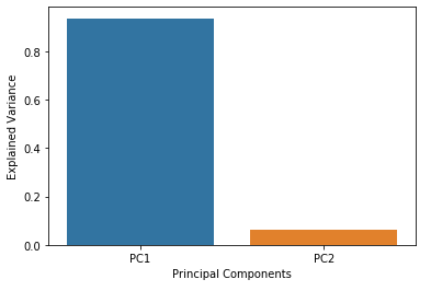
The aim of PCA is to explain the variance within the original dataset as much as possible by using less features (or columns). The new derived features are called principal components. The order of principal components is determined according to the fraction of variance of original dataset they explain.

The principal components are linear combinations of the features of original dataset.

The advantage of PCA is that a significant amount of variance of the original dataset is retained using much smaller number of features than the original dataset. Principal components are ordered according to the amount of variance they explain.

---

Source: https://towardsdatascience.com/11-most-common-machine-learning-algorithms-explained-in-a-nutshell-cc6e98df93be

References:

Tuesday, July 28, 2020